Overview
This tutorial describes the theory of operation of the hydrodynamics plugin. It's heavily based on [3], and we recommend to read the full paper for a deeper understanding of its theory.
Understanding Hydrodynamic Forces
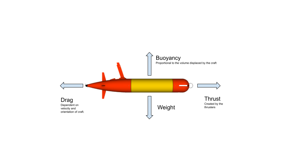
The behavior of a moving body through water is different from the behavior of a ground based vehicle. In particular bodies moving underwater experience many more forces derived from drag, buoyancy and lift. The way these forces act on a body can be seen in the following diagram:
The hydrodynamics plugin
To approximate the motion of the vehicle in the ocean environment, we adapt Fossen’s six degree-of-freedom robot-like vectorial model for marine craft [2] expressed as
$$M ẍ + C(ẋ)ẋ + D(ẋ)ẋ = F$$
where M is the inertia matrix (including added mass), C(ẋ) is the Coriolis-centripetal matrix, D(ẋ) is the damping matrix, and ẋ is the velocity six-vector.
If present, ocean current is approximated by using the relative velocity ẋr = ẋ − vc:
$$M ẍ + C(ẋ_r)ẋ_r + D(ẋ_r)ẋ_r = F$$
Added mass and Coriolis (M and C terms) are handled by the physics engine via the SDF <fluid_added_mass> tag on the link’s <inertial> element. This provides implicit integration that is unconditionally stable. See the SDF specification for details.
Hydrodynamic damping (D term) is handled by the Hydrodynamics plugin. This includes forces due to radiation-induced potential damping, skin friction, wave drift damping, vortex shedding and lifting forces. These effects are aggregated in the damping matrix. The user defines the vessel’s damping characteristics through SDF parameters using the SNAME naming convention. During each time step, the plugin computes the damping force using the velocity relative to the ocean current and applies it to the vessel.
When both <fluid_added_mass> and an ocean current are present, the plugin also applies a Coriolis correction so that the added-mass Coriolis force uses the relative velocity rather than the absolute velocity.
The next table summarizes the available SDF parameters for the plugin.
| Parameter | Description |
|---|---|
| <xUabsU> | Quadratic drag in surge |
| <xU> | Linear drag in surge |
| <yVabsV> | Quadratic drag in sway |
| <yV> | Linear drag in sway |
| <zWabsW> | Quadratic drag in heave |
| <zW> | Linear drag in heave |
| <kPabsP> | Quadratic drag in roll |
| <kP> | Linear drag in roll |
| <mQabsQ> | Quadratic drag in pitch |
| <mQ> | Linear drag in pitch |
| <nRabsR> | Quadratic drag in yaw |
| <nR> | Linear drag in yaw |
| <default_current> | Default ocean current vector |
A simple example
Let's download the provided buoyant_cylinder.sdf world and run to see an example of a cylinder with three plugins attached:
- Buoyancy: It will make the cylinder float on the surface of the water.
- Hydrodynamics: It will simulate the damping generated by the fluid surrounding the cylinder.
- Trajectory follower: It will apply some force to move the cylinder one meter in the positive
Xdirection.
Observe how the cylinder does not sink, and slowly makes its way until it reaches (1, 0, 0) in world coordinates.
Now let's make a change in the hydrodynamics parameters. Considering that the model only moves in X direction (or surge in the maritime terminology), we're going to reduce the value of <xUabsU> and <xU> parameters. Update these parameters to:
And run Gazebo again:
Notice how the vehicle does not stop at the 1 meter mark. Instead, the cylinder stops further. This is because we lowered the linear and quadratic drag in the direction that the model is moving.
Let's now try the opposite. Go ahead and update the same parameters to the following values:
And run Gazebo:
See how slow the cylinder moves. With these set of parameters we increased the damping in the surge axis, causing the vehicle to slowly move towards its goal.
Experimental - How to tune the parameters
The hydrodynamics plugin requires a number of parameters to model the drag behavior of underwater vehicles. The added mass is specified separately using the SDF <fluid_added_mass> tag. This section describes methods to determine these parameters. Note these parameters need to be tested and possibly tweaked to guarantee model stability.
Added mass
A python library called Capytaine can be used to determine the added mass matrix of your vehicle. Capytaine enables the user to import a mesh (.stl), define a set of linear potential flow problems and solve these using the included Boundary Element Method (BEM) solver.
Capytaine is typically used to model the interaction between floating bodies and waves, however it can be applied to ROVs by setting the wave frequency and free surface both to infinity (this assumes that the added mass is approximately constant since the ROV does not operate near the wave zone and that it operates in infinitely deep water respectively) [1] (p.14), [2] (p.18).
Furthermore, it is recommended to use a simplified mesh when computing the added mass with Capytaine, since a complex mesh is computationally prohibitive.
Once you have the added mass values, specify them using the <fluid_added_mass> tag in your link's <inertial> element. For example, for diagonal added mass:
Note that <fluid_added_mass> uses positive values, unlike the deprecated plugin parameters which used the negative Fossen sign convention.
Recommended added mass configuration by physics engine
| Physics Engine | Recommended Method | Notes |
|---|---|---|
| DART | Native <fluid_added_mass> in SDF <inertial> + <disable_added_mass>true in plugin | Unconditionally stable, full 6x6 matrix, implicit Coriolis |
| Bullet-Featherstone | Plugin parameters (<xDotU>, etc.) | Native added mass not supported; plugin is the only option |
| Bullet (classic) | Plugin parameters (<xDotU>, etc.) | Native added mass not supported; plugin is the only option |
| MuJoCo | Plugin parameters (<xDotU>, etc.) | Native added mass not supported; plugin is the only option |
Warning: Do not set added mass in both places simultaneously. If both <fluid_added_mass> and plugin parameters are active, forces are double-counted.
Linear and quadratic damping
Computing the linear and quadratic damping coefficients is generally not possible using computational analysis and is usually done experimentally [1] (p.28). If determining the damping coefficients experimentally is not feasible, the same method described by Berg2012 can be used to estimate these values from a similar ROV [1] (p.28-31).
References
[1] BERG, V. Development and Commissioning of a DP system for ROV SF 30k, 2012.
[2] FOSSEN , T. I. Lecture notes: Ttk 4190 guidance, navigation and control of vehicles, February 2021.
[3] BINGHAM, B. et al., Toward Maritime Robotic Simulation in Gazebo, Oceans Conference, 2019.